Initial Results
To start the analysis, quadrant A-X was chosen as a consequence of using the ABC-XYZ matrix of all product clusters of the company, since it presents two advantages:
-
A-type products have a great impact upon the company's success, which translates to greater overall costs, so reducing these prove more advantageous.
-
X-type products have stable demand variation, so changes in its production plan present a very reduced risk.
After running the Optimization Model, over the A-X quadrant, a resulting set of Coverage Times was obtained, as be seen in following image.
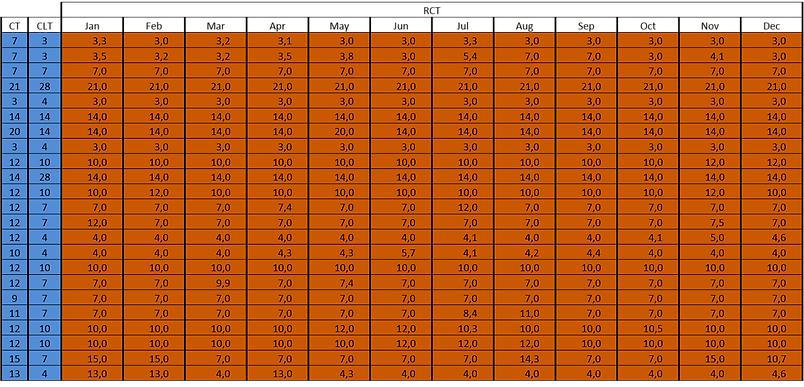
This is the format of the proposed model's results. on the left, with a blue background, are the maximum and minimum limits, respectively, for the model's results. Once the model was complete, the remaining A type quadrants were also analyzed. With these new Coverage Times reductions in litres are presented.
Results Validation
Before attempting to evaluate the financial gain, one must study the results' quality, Such is done graphically, and mathematically.
The initial approach compares the daily Sales and Existences records with the suggested stock levels (CT, CLT, MCT, SSAlt and RCT). Considering the results are isolated from month to month, with the exception of MCT (which depends on the analogous months results), the graphical representation reveals the 3 analogous months simultaneously. An example is depicted below.

The image above represents one of the four categorized behaviours:
-
No Improvement - where CLT is greater than CT, so the resulting CTs remain the same.
The remaining types of behaviours are named and described as follows:
-
Clear Improvement - where RCT's stock level is substantually lower than the initial CT and demand is stil clearly not high enough to risk the occurence of a stock-out.
-
Slight Excesses - the product's Sales record a rare amount of instants where it is greater than the suggested levels. As such, implementing this strategy, must be done as a carefully monitored process.
-
Order Response - the product's Sales have an erratic behaviour, hence the the implementation a lower Safety Stock level brings reduced improvements in comparison with products with a more stable demand.
Secondly, the mathematical analysis presents the Stock Service Level with the implemented model, validated on a daily basis.
A - X

A - Y

A - Z

Scenario Analysis
Once the initial results of the model were validated, they were monetized and compared with a set of scenarios, deepening the understanding and results of the proposed model.
The first step in creating the scenarios was the selection of a variable parameter/s.
-
Varying CT is the objective of the model.
-
Real Demand and Forecasts are historic, therefore unvarying, records.
-
Concluding that CLT is the only variable worth exploring
-
Because CLT depends on its two components, a certain bidimensionality is observable in the scenarios.
-
The first scenario, is the Material Restriction Scenario. Assuming that the material's requirements are permanently assured, their internal LT's value is 1. By changing the product's MLT value to 1, this scenario becomes possible to simulate.
If a product's CLT changes when applying this scenario, they are selected for the scenario's analysis. As such, only three products were selected.

This scenario presents virtually no implementation costs, and since it presents improvemnts over the initial results, it's safe to consider it viable.
The second scenario regards the PLT. The criteria selection for this scenario are more numerous and the testing is more extensive. The criteria are as follows:
-
CLT must be defined by PLT.
-
CLT must be greater than the average of all product's CLT.
-
The product in question must be glass bottled beer. This restriction is imposed, because only this type of product has lines which can be adapted to produce it.
As such, only 5 product fit the selection criteria, and they are represented in the figure below:

Now all that is left is calculating the return on investment, for adapting any one production line for these products.

The acceptable RoI for Unicer is two years. Because no product has such a quik return, this scenario is not deemed applicable.
The last scenario is a combination of the first and second scenario's criteria and modifications.
The list of selected products, the obtained improvement and return of investment is in the figure below.

It's possible to see that no product is affected by both scenarios, making the decision of applying one of the scenarios independent from the application of the other.